本文介绍logistic回归的相关知识，以及用R语言来实现逻辑回归，解决分类的问题

二分类logistic回归介绍

logistic回归是用来解决分类问题的统计或机器学习模型，这里我们只介绍最简单的 二分类logistic回归 。这个模型经常用于识别垃圾邮件、判断病人是否有疾病、预测客户是否买房等等。

1. logistic函数和logit变换

现在普及两个基础函数：

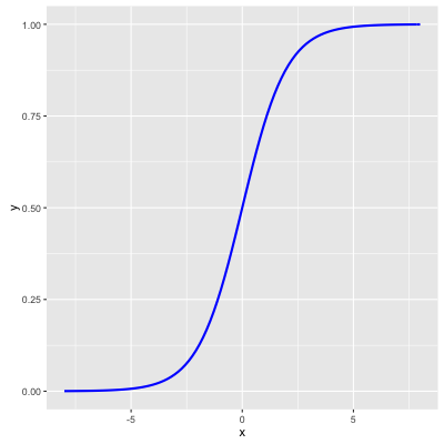
logistic函数。$f(x)=\frac{1}{1+e^{-x}}$
logit变换。$logit P=ln(\frac{P}{1-P})$

有趣的是，logit变换是logistic函数的反函数 ，$f(x)=\frac{1}{1+e^{-x}}$ , $g(x)=ln(\frac{P}{1-P})$, $g(f(x))=ln(\frac{\frac{1}{1+e^{-x}}}{1-\frac{1}{1+e^{-x}}})=x$

library(ggplot2)
logistic_fun = function(x){1/(1+exp(-x))}
ggplot(data.frame(x = c(-8,8)),aes(x)) +
  stat_function(fun = logistic_fun,
                color = "blue",
                size = 1)

logistic函数图形如下，它是 Sigmoid函数 最重要的代表：

2. 二分类logistic回归详解

比如要解决二分类问题，我们最先想到的是建立个线性回归方程 $y = \mathbf {w}^{T}\mathbf {x} + b$ 。但是这个回归方程 $y$ 的取值范围不受约束，而 $y$在分类问题中应该只有 1 和 0 两个取值(1代表正例，0代表反例)，自然想到将它代入logistic函数，得 $y = \frac{1}{1+e^{-(\mathbf {w}^{T}\mathbf {x}+b)}}$ , $y$ 取值在0～1之间。

上式推导:

$\ln \frac{y}{1-y} = \frac{\frac{1}{1+e^{-(\mathbf {w}^{T}\mathbf {x} + b)}}}{1-\frac{1}{1+e^{-(\mathbf {w}^{T}\mathbf {x} + b)}}}=\mathbf {w}^{T}\mathbf {x} + b$

这样的话，我们的 logistic回归方程 为

$\ln \frac{y}{1-y} =\mathbf {w}^{T}\mathbf {x} + b$

odds和log odds

如 $y$ 表示样本取1的概率(正例)，$1-y$ 表示样本取0的概率(反例)。则 $\frac{y}{1-y}$ 代表样本取正例的相对可能性，记为 odds ，log odds 是 $ln\frac{y}{1-y}$ ，称为 对数几率

极大似然估计

有了回归方程后就可以用 极大似然估计进行参数估计

若将 回归方程 中的 $y$ 当作后验概率，则回归方程可写为

$\ln \frac{p(y=1|\mathbf{x})}{p(y=0|\mathbf{x})}=\mathbf{w}^{T}\mathbf{x}+b$

$y$ 和 $1-y$ 分别写为

$p(y=1|\mathbf{x})=\frac{1}{1+e^{-(\mathbf{w}^{T}\mathbf{x}+b)}}$ $p(y=0|\mathbf{x})=\frac{e^{-(\mathbf{w}^{T}\mathbf{x}+b)}}{1+e^{-(\mathbf{w}^{T}\mathbf{x}+b)}}$

假设有n个独立的训练样本，$(x_{1},y_{1}),(x_{2},y_{2})…(x_{n},y_{n})$ , $y\in (0,1)$

设 $p_{i}=P(y_{i}=1\mid x_{i})$ 是 $y_{i}=1$ 的概率，那么 $y_{i}=0$ 的概率就是 $1-p_{i}$

任意一个观测值 $(x_{i},y_{i})$ 出现的概率是

$P(x_{i},y_{i})=p_{i}^{y_{i}}(1-p_{i})^{1-y_{i}}$

容易构造 似然函数

$L(w)=\prod_{i=1}^{m}P(x_{i},y_{i})$

取对数即得到 对数似然函数

$lnL(w)=\sum_{i=1}^{m}[y_{i}lnp_{i}+(1-y_{i})ln(1-p_{i})]$

接下来的问题就是最大化似然函数来求解参数。这里就要用到一些经典的 数值优化算法

3. 参数求解方法

梯度下降法(gradient descent)

1	geom_segment(aes(5,25,xend=4,yend=16),arrow=arrow(),size=1,color="red")

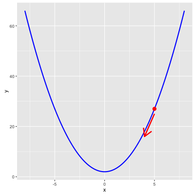
简单介绍一下梯度下降法。梯度下降法是一种寻找局部最优的算法。以上图的抛物线 $y=x^{2}+2$ 为例，假设我们选定初始点(5,27)，对于这个点对 $x$ 求偏导数为 $2x$ ，即4。沿着+4的方向，y值会变大，称为 梯度上升；沿着-4的方向，y值变小，称为 梯度下降 。

梯度下降法有两个关键：

初始点的选择
下降的速度

未完待续…

牛顿法(newton method)

牛顿法是二阶收敛，相比一阶收敛的梯度下降法能更快的找到最优解

拟牛顿法(newton-raphson method)

5. R语言实例

# logistic regression
library(dplyr)
library(ggplot2)
library(tidyr)
iris_total = iris %>%
  filter(
    Species %in% c("versicolor","virginica")
  )
head(iris_total)
# logistic model
logit.fit = glm(Species ~ Petal.Width + Petal.Length,
                family = binomial(link = "logit"),
                data = iris_total)
# prediction
logit.prediction = ifelse(predict(logit.fit) > 0,
                          "virginica","versicolor")
iris_total$logitSpecies = logit.prediction
# gather species and logitspecies
x = iris_total %>%
  gather(
    models,
    Species,
    Species:logitSpecies
  )

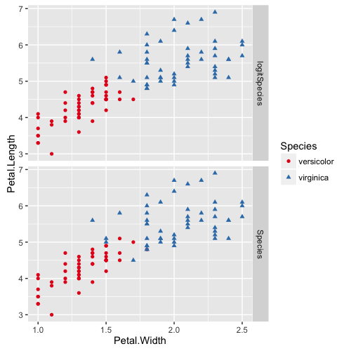
x数据集如下，其中 models 为 Species 的是花瓣真实分类， logitSpecies 代表 logistic回归 预测的分类

> head(x)
  Sepal.Length Sepal.Width Petal.Length Petal.Width  models    Species
1          7.0         3.2          4.7         1.4 Species versicolor
2          6.4         3.2          4.5         1.5 Species versicolor
3          6.9         3.1          4.9         1.5 Species versicolor
4          5.5         2.3          4.0         1.3 Species versicolor
5          6.5         2.8          4.6         1.5 Species versicolor
6          5.7         2.8          4.5         1.3 Species versicolor

下图比较预测值和真实值的区别，可以看到预测的结果还是不错的～

p = ggplot(data = x,
           aes(Petal.Width,Petal.Length,
               color = Species,
               shape = Species)) +
  geom_point() +
  scale_color_brewer(palette = "Set1") +
  facet_grid(models~.)
p

> table(iris_total$Species,iris_total$logitSpecies)

             versicolor virginica
  setosa              0         0
  versicolor         47         3
  virginica           3        47

一共100个样本，分类错误样本为6个，正确率94%