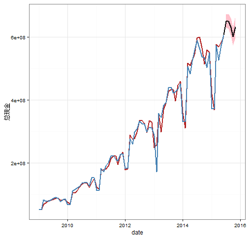
背景是最近预估公司的总现金,在这里记录使用ARIMA模型预测的流程
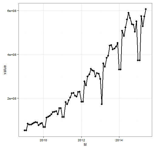
原始时间序列
加载包
1 | library(TSA) |
原始时间序列
1 | setwd("C:/Users/lixinyao_bj/Desktop/program/增值预估") |
平稳性
单位根检验
原假设:非平稳
1 | > adf.test(MXJts) |
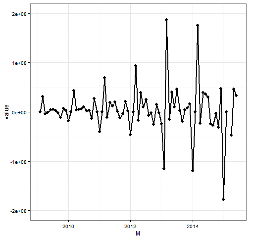
差分
1 | MXJtsDiff = diff(MXJts) |
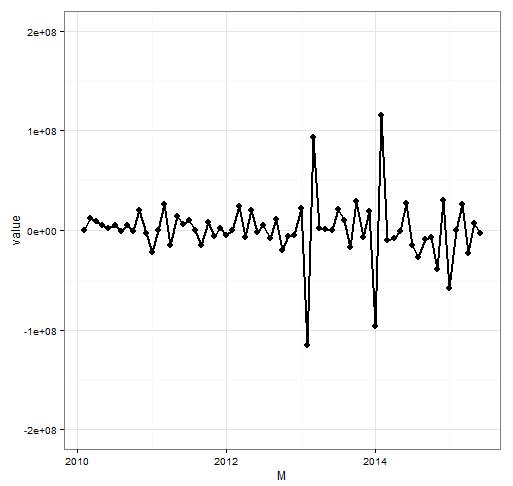
一阶一次差分序列
1 | ggplot(mydata2,aes(M,value)) + geom_line(size=1) + geom_point(size=3) + theme_bw() + ylim(-2*10^8,2*10^8) |
12阶差分
差分后效果很好
1 | MXJtsDiff2 = diff(MXJtsDiff,lag=12) |
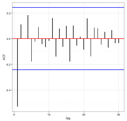
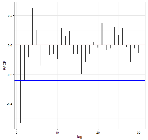
相关性
ACF
1 | qacf = function(x, conf.level = 0.95) { |
PACF
1 | qpacf = function(x, conf.level = 0.95) { |
定阶
auto辅助定阶
auto.arima(log(MXJts))
采用bestAIC来定阶
1 | get.best.arima = function(x.ts, maxord = c(1,1,1,1,1,1)) |
结果中的值就是ARIMA(p,d,q,P,D,Q)
残差检验
1 | y=Arima(log(MXJts),order=c(bae[1],bae[2],bae[3]),seasonal=c(bae[4],bae[5],bae[6]),method="ML") |
预测
1 | z = forecast(y,level=c(1,95)) |